简介 前几篇博客文章介绍了MATLAB绘图的基本操作,本篇博客接下来介绍通过Python中的Matplotlib库进行图像的绘制。
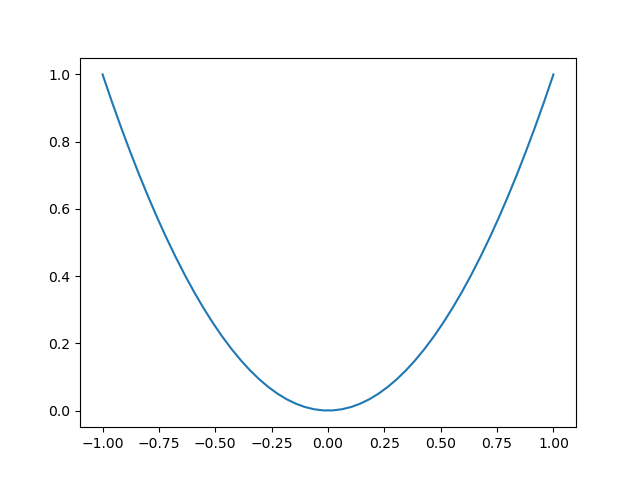
一、基本绘图 绘制y=x^2的图线:
1
2
3
4
5
6
7
8
import matplotlib.pyplot as pltimport numpy as npx = np.linspace(-1 , 1 , 50 ) y = x**2 plt.plot(x, y) plt.show()
绘图结果:
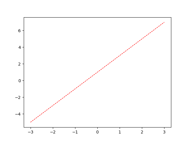
二、窗口 1 2 3 4 5 6 7 8 9 10 11 12 13 14 15 16 17 18 import matplotlib.pyplot as pltimport numpy as npx = np.linspace(-3 , 3 , 50 ) y1 = 2 *x+1 y2 = x**2 plt.figure() plt.plot(x, y1, color='red' , linewidth=1.0 , linestyle='--' ) plt.figure(num=3 , figsize=(8 , 5 )) plt.plot(x, y2) plt.show()
在这里,我们可以通过两个窗口显示两个函数的图像。最基本的窗口语句为plt.figure(),语句内包含几个参数,具体可参阅matplotlib官方文档。在注释行中我们还加入了多函数显示方法,一个图像窗口中有可以显示两个图线。
函数y=2x+1:
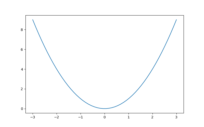
函数y=x^2:
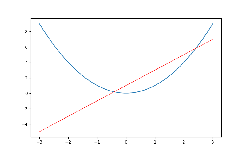
两个函数同时显示:
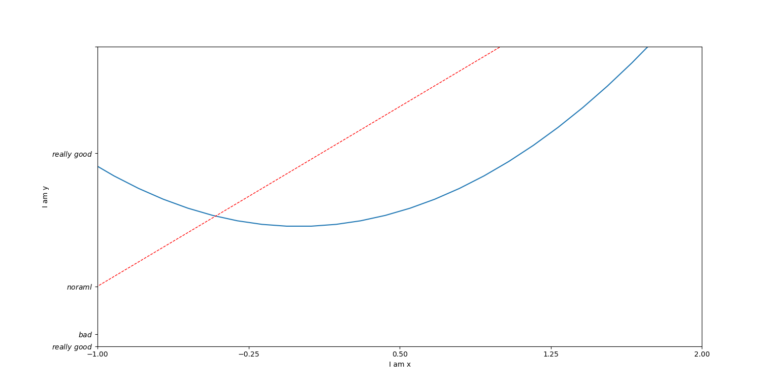
三、设置坐标轴 1 2 3 4 5 6 7 8 9 10 11 12 13 14 15 16 17 18 19 20 21 22 23 24 25 import matplotlib.pyplot as pltimport numpy as npx = np.linspace(-3 , 3 , 50 ) y1 = 2 *x+1 y2 = x**2 plt.figure(num=1 , figsize=(8 , 5 )) plt.plot(x, y2) plt.plot(x, y1, color='red' , linewidth=1.0 , linestyle='--' ) plt.xlim((-1 , 2 )) plt.ylim((-2 , 3 )) plt.xlabel('I am x' ) plt.ylabel('I am y' ) new_ticks = np.linspace(-1 , 2 , 5 ) print(new_ticks) plt.xticks(new_ticks) plt.yticks([-2 , -1.8 , -1 , 1.22 , 3 ], [r'$really\ good$' , r'$bad$' , r'$noraml$' , r'$really\ good$' ]) plt.show()
在这里通过plt.x/ylim()函数将图中显示的坐标范围固定,同时通过plt.x/ylabel()函数对坐标轴进行标识;在程序的最后针对坐标轴的间隔进行调整,通过plt.x/yticks函数实现,若想实现指定的间隔,需要创建一个一维数组。
绘图结果:
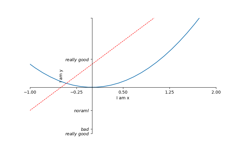
1 2 3 4 5 6 7 8 9 10 11 12 13 14 15 16 17 18 19 20 21 22 23 24 25 26 27 28 29 30 31 32 33 34 import matplotlib.pyplot as pltimport numpy as npx = np.linspace(-3 , 3 , 50 ) y1 = 2 *x+1 y2 = x**2 plt.figure(num=1 , figsize=(8 , 5 )) plt.plot(x, y2) plt.plot(x, y1, color='red' , linewidth=1.0 , linestyle='--' ) plt.xlim((-1 , 2 )) plt.ylim((-2 , 3 )) plt.xlabel('I am x' ) plt.ylabel('I am y' ) new_ticks = np.linspace(-1 , 2 , 5 ) print(new_ticks) plt.xticks(new_ticks) plt.yticks([-2 , -1.8 , -1 , 1.22 , 3 ], [r'$really\ good$' , r'$bad$' , r'$noraml$' , r'$really\ good$' ]) ax = plt.gca() ax.spines['right' ].set_color('none' ) ax.spines['top' ].set_color('none' ) ax.xaxis.set_ticks_position('bottom' ) ax.yaxis.set_ticks_position('left' ) ax.spines['bottom' ].set_position(('data' , 0 )) ax.spines['left' ].set_position(('data' , 0 )) plt.show()
在这里主要采用ax.spines[‘right’].set_color(‘none’)语句关闭图中右边框的显示,ax.xaxis.set_ticks_position(‘bottom’)语句表示下边框的显示;ax.spines[‘bottom’].set_position((‘data’, 0))语句将下边框移动到y=0的位置,同理ax.spines[‘left’].set_position((‘data’, 0))语句将左边框移动到x=0的位置。
绘图结果:
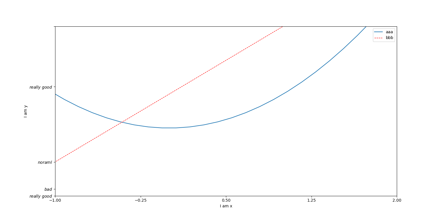
四、图例(legend) 1 2 3 4 5 6 7 8 9 10 11 12 13 14 15 16 17 18 19 20 21 22 23 24 25 26 27 import matplotlib.pyplot as pltimport numpy as npx = np.linspace(-3 , 3 , 50 ) y1 = 2 *x+1 y2 = x**2 plt.figure() plt.xlim((-1 , 2 )) plt.ylim((-2 , 3 )) plt.xlabel('I am x' ) plt.ylabel('I am y' ) new_ticks = np.linspace(-1 , 2 , 5 ) print(new_ticks) plt.xticks(new_ticks) plt.yticks([-2 , -1.8 , -1 , 1.22 , 3 ], [r'$really\ good$' , r'$bad$' , r'$noraml$' , r'$really\ good$' ]) l1, = plt.plot(x, y2, label='up' ) l2, = plt.plot(x, y1, color='red' , linewidth=1.0 , linestyle='--' ) plt.legend(handles=[l1, l2, ], labels=['aaa' , 'bbb' ], loc='best' ) plt.show()
在这里绘图表示成l1和l2,图例(legend)的设置采用语句plt.legend(),参数handles表示绘制的图线,labels表示图线的名称,loc表示图例的位置,详细参数设置请参考matplotlib官方文档资料。
绘图结果:
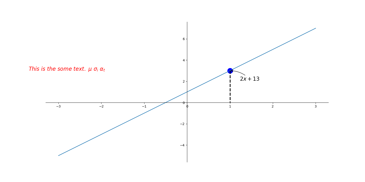
五、为图中函数添加公式和注解 1 2 3 4 5 6 7 8 9 10 11 12 13 14 15 16 17 18 19 20 21 22 23 24 25 26 27 28 29 30 31 32 33 import matplotlib.pyplot as pltimport numpy as npx = np.linspace(-3 , 3 , 50 ) y = 2 *x+1 plt.figure(num=1 , figsize=(8 , 5 )) plt.plot(x, y) ax = plt.gca() ax.spines['right' ].set_color('none' ) ax.spines['top' ].set_color('none' ) ax.xaxis.set_ticks_position('bottom' ) ax.yaxis.set_ticks_position('left' ) ax.spines['bottom' ].set_position(('data' , 0 )) ax.spines['left' ].set_position(('data' , 0 )) x0 = 1 y0 = 2 *x0 + 1 plt.scatter(x0, y0, s=250 , color='b' , ) plt.plot([x0, x0], [y0, 0 ], 'k--' , lw=2.5 ) plt.annotate(r'$2x+1%s$' , xy=(x0, y0), xycoords='data' , xytext=(+30 , -30 ), textcoords='offset points' , fontsize=16 , arrowprops=dict(arrowstyle='->' , connectionstyle='arc3, rad=.2' )) plt.text(-3.7 , 3 , r'$This\ is\ the\ some\ text.\ \mu\ \sigma_i\ \alpha_t$' , fontdict={'size' : 16 , 'color' : 'r' }) plt.show()
在这里,method1通过绘制散点图的方法绘制出了x0=1处对应的直线上的点,将公式以箭头的方式指向该点,使用的语句:plt.annotate();method2则给出了在图中加入文字的方式,使用的语句:plt.text。
绘图结果:
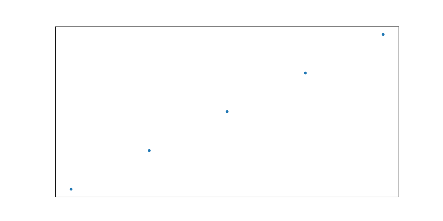
六、绘制散点图 1 2 3 4 5 6 7 8 9 10 11 12 13 14 15 16 17 import matplotlib.pyplot as pltimport numpy as npn = 1024 X = np.random.normal(0 , 1 , n) Y = np.random.normal(0 , 1 , n) T = np.arctan2(Y, X) plt.scatter(np.arange(5 ), np.arange(5 )) plt.xticks(()) plt.yticks(()) plt.show()
绘图结果:
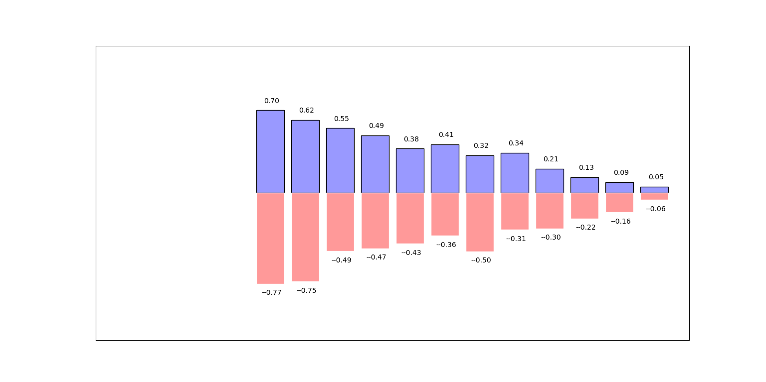
七、柱状图 1 2 3 4 5 6 7 8 9 10 11 12 13 14 15 16 17 18 19 20 21 22 23 24 25 import matplotlib.pyplot as pltimport numpy as npn = 12 X = np.arange(n) Y1 = (1 - X/float(n))*np.random.uniform(0.5 , 1.0 , n) Y2 = (1 - X/float(n))*np.random.uniform(0.5 , 1.0 , n) plt.bar(X, +Y1, facecolor='#9999ff' , edgecolor='black' ) plt.bar(X, -Y2, facecolor='#ff9999' , edgecolor='white' ) for x, y in zip(X, Y1): plt.text(x + 0.04 , y + 0.05 , '%.2f' % y, ha='center' , va='bottom' ) for x, y in zip(X, Y2): plt.text(x + 0.04 , -y - 0.05 , '-%.2f' % -y, ha='center' , va='top' ) plt.xlim(-5 , n) plt.xticks(()) plt.ylim(-1.25 , 1.25 ) plt.yticks(()) plt.show()
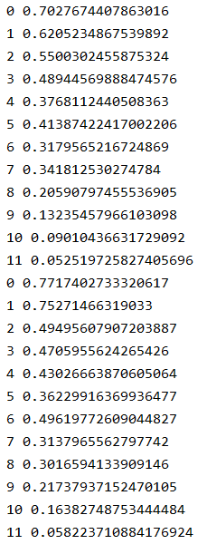
本程序涉及的关键点大概有两个:绘制柱状图和显示柱状图的值。绘制柱状图使用plt.bar()语句,其中facecolor表示柱状图柱的颜色,edgecolor表示柱状图柱的边缘线的颜色;在柱状图上显示值,这里采用了for…zip()循环,在这里可以打印出执行该循环的结果:
可以看到,此时已将x的值和y的值一一对应,不再是两个一维向量的形式,这样plt.text()语句就可以通过for…zip()输出的参数对柱状图进行数值的标注。
绘图结果:
在这里有另外一个较为简单的程序可以参考:
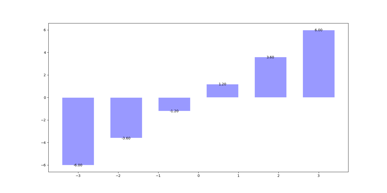
1 2 3 4 5 6 7 8 9 10 11 12 13 14 15 import matplotlib.pyplot as pltimport numpy as npx = np.linspace(-3 , 3 , 6 ) y = x*2 plt.figure() plt.bar(x, y, facecolor='#9999ff' , edgecolor='white' ) for X, Y in zip(x, y): print(x, y) print(X, Y) plt.text(X, Y+0.125 , '%.2f' % Y, ha='center' , va='top' ) plt.show()
绘图结果:
注:’%.2f’显示保留两位小数的浮点数,类似地’%.3f’是保留3位小数,’%.2f’%Y表示将Y显示保留两位小数。
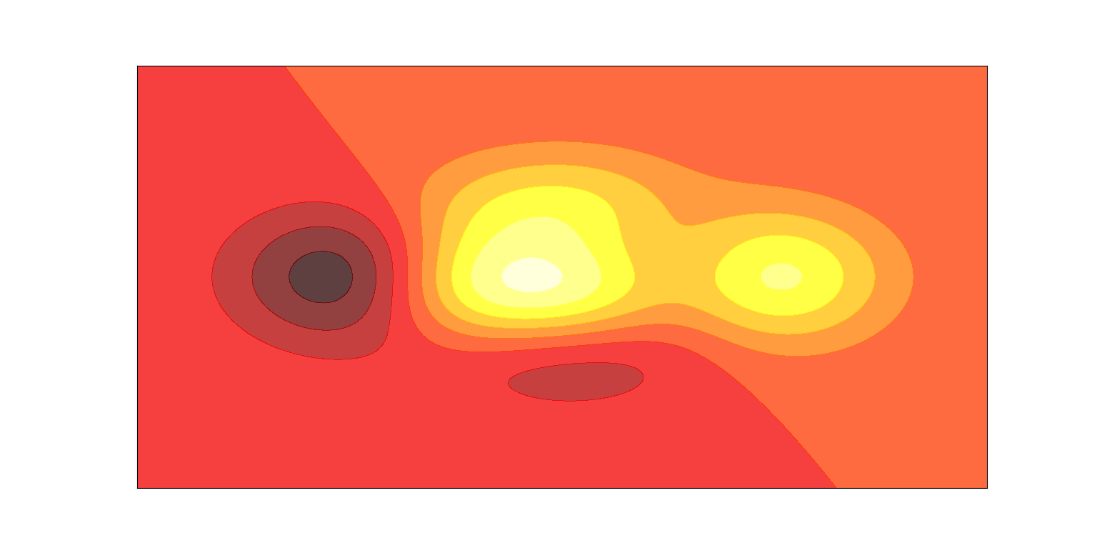
八、绘制等高线 1 2 3 4 5 6 7 8 9 10 11 12 13 14 15 16 17 18 19 import matplotlib.pyplot as pltimport numpy as npdef f (x, y) : return (1 -x/2 +x**5 +y**3 )*np.exp(-x**2 -y**2 ) n = 256 x = np.linspace(-3 , 3 , n) y = np.linspace(-3 , 3 , n) X, Y = np.meshgrid(x, y) plt.contourf(X, Y, f(X, Y), 8 , alpha=0.75 , cmap=plt.cm.hot) plt.xticks(()) plt.yticks(()) plt.show()
绘制等高线使用plt.contourf()语句,绘图结果:
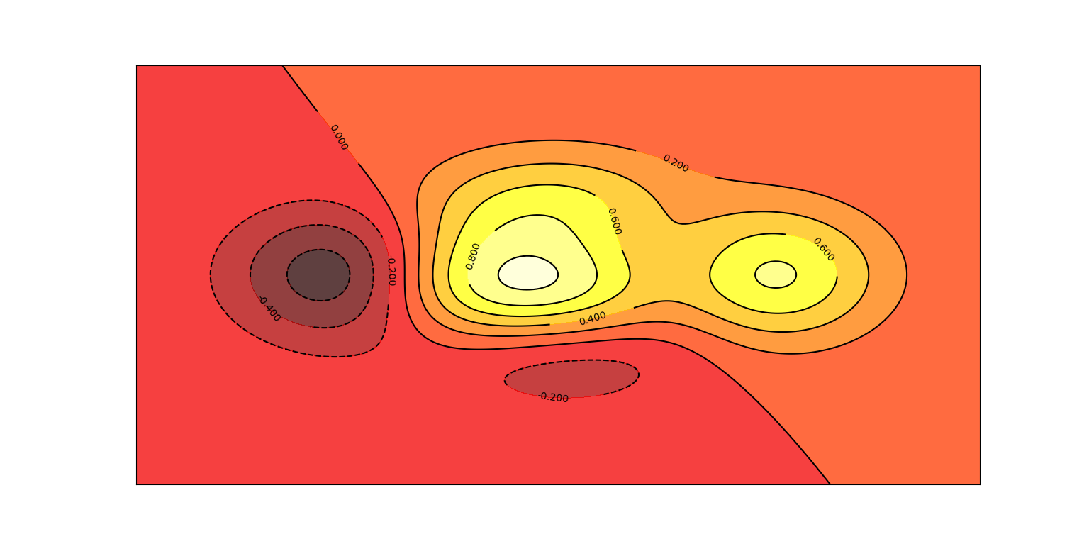
我们可以看到,等高线图已经绘制出,但是没有等高线和数值,因此可以在该程序基础上添加以下程序:
1 2 C = plt.contour(X, Y, f(X, Y), 8 , colors='black' , linewidth=0.5 ) plt.clabel(C, inline=True , fontsize=10 )
注:该程序需要添加到plt.contourf()语句之后。
绘图结果:
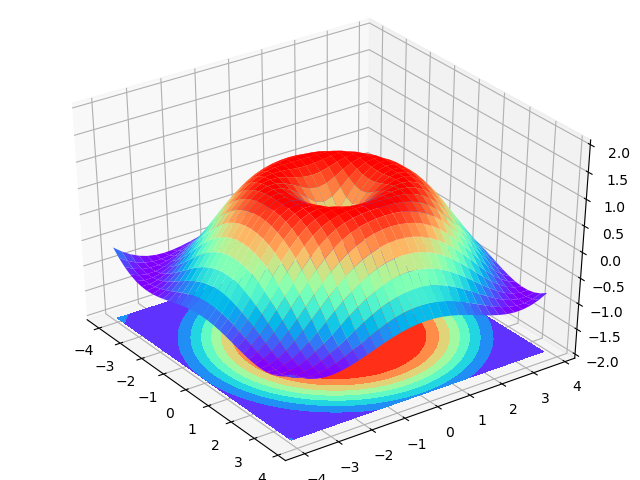
九、绘制3D图 1 2 3 4 5 6 7 8 9 10 11 12 13 14 15 16 17 18 19 20 21 import numpy as npimport matplotlib.pyplot as pltfrom mpl_toolkits.mplot3d import Axes3Dfig = plt.figure() ax = Axes3D(fig) X = np.arange(-4 , 4 , 0.25 ) Y = np.arange(-4 , 4 , 0.25 ) X, Y = np.meshgrid(X, Y) R = np.sqrt(X**2 +Y**2 ) Z = np.sin(R) ax.plot_surface(X, Y, Z, rstride=1 , cstride=1 , cmap=plt.get_cmap('rainbow' )) ax.contourf(X, Y, Z, zdir='z' , offset=-2 , cmap='rainbow' ) ax.set_zlim(-2 , 2 ) plt.show()
绘图结果:
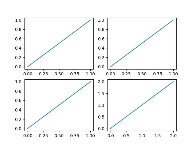
十、多图绘制 1 2 3 4 5 6 7 8 9 10 11 12 13 14 15 16 17 import matplotlib.pyplot as pltplt.figure() plt.subplot(2 , 2 , 1 ) plt.plot([0 , 1 ], [0 , 1 ]) plt.subplot(2 , 2 , 2 ) plt.plot([0 , 1 ], [0 , 1 ]) plt.subplot(2 , 2 , 3 ) plt.plot([0 , 1 ], [0 , 1 ]) plt.subplot(2 , 2 , 4 ) plt.plot([0 , 2 ], [0 , 2 ]) plt.show()
绘图结果:
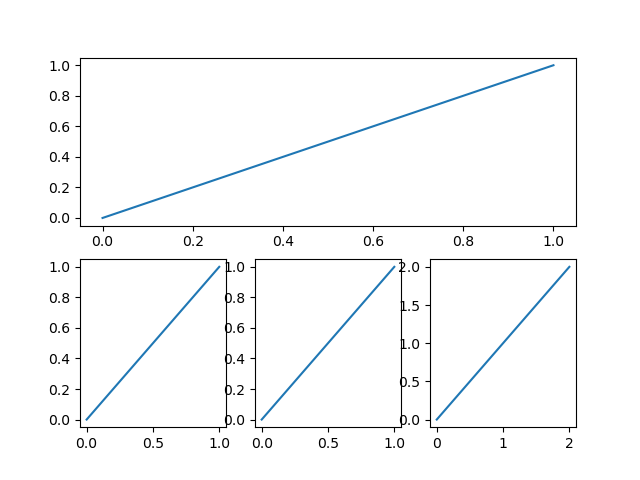
1
2
3
4
5
6
7
8
9
10
11
12
13
14
15
16
17
import matplotlib.pyplot as pltplt.figure() plt.subplot(2 , 1 , 1 ) plt.plot([0 , 1 ], [0 , 1 ]) plt.subplot(2 , 3 , 4 ) plt.plot([0 , 1 ], [0 , 1 ]) plt.subplot(2 , 3 , 5 ) plt.plot([0 , 1 ], [0 , 1 ]) plt.subplot(2 , 3 , 6 ) plt.plot([0 , 2 ], [0 , 2 ]) plt.show()
绘图结果:
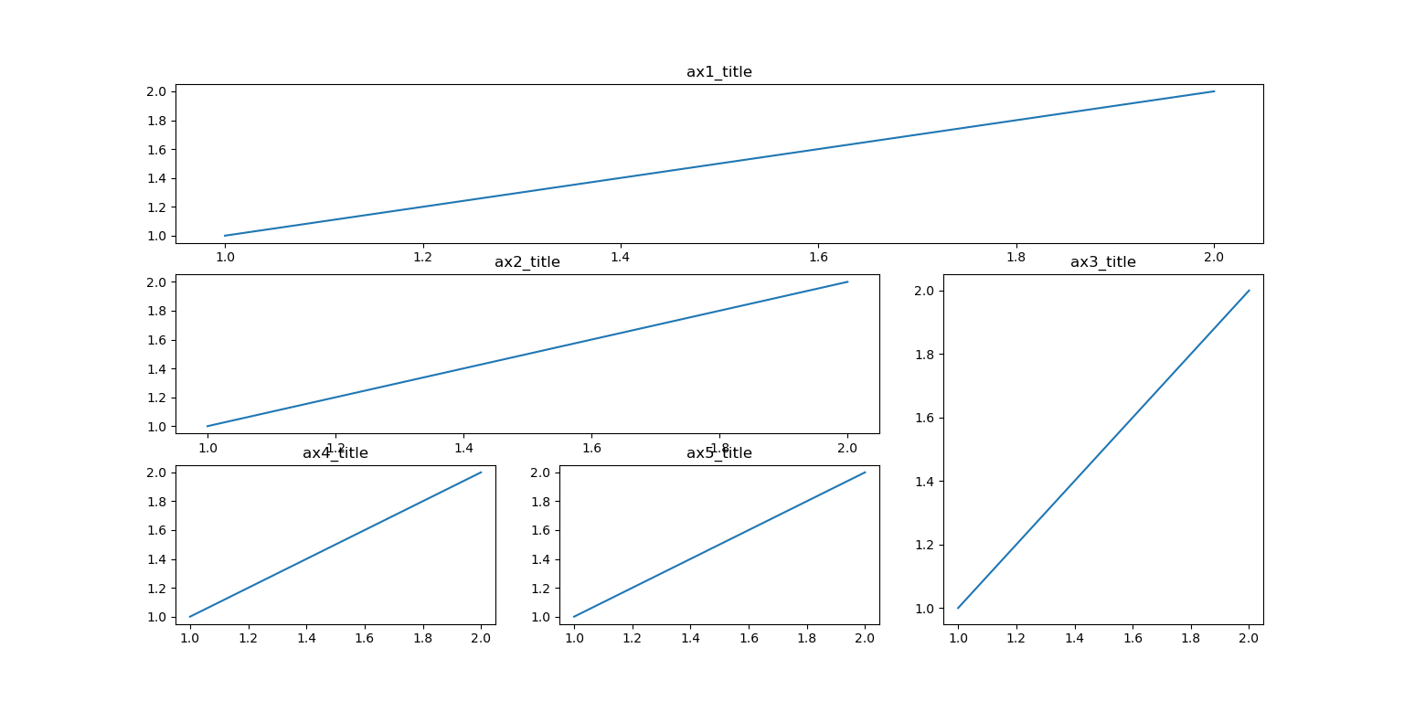
3、subplot2grid 1 2 3 4 5 6 7 8 9 10 11 12 13 14 15 16 17 18 19 20 21 22 23 24 25 import matplotlib.pyplot as pltplt.figure() ax1 = plt.subplot2grid((3 , 3 ), (0 ,0 ), colspan=3 , rowspan=1 ) ax1.plot([1 , 2 ], [1 , 2 ]) ax1.set_title('ax1_title' ) ax2 = plt.subplot2grid((3 , 3 ), (1 , 0 ), colspan=2 , ) ax2.plot([1 , 2 ], [1 , 2 ]) ax2.set_title('ax2_title' ) ax3 = plt.subplot2grid((3 , 3 ), (1 , 2 ), rowspan=2 ) ax3.plot([1 , 2 ], [1 , 2 ]) ax3.set_title('ax3_title' ) ax4 = plt.subplot2grid((3 , 3 ), (2 , 0 )) ax4.plot([1 , 2 ], [1 , 2 ]) ax4.set_title('ax4_title' ) ax5 = plt.subplot2grid((3 , 3 ), (2 , 1 )) ax5.plot([1 , 2 ], [1 , 2 ]) ax5.set_title('ax5_title' ) plt.show()
plt.subplot2grid()语句中,第一个参数(3, 3)代表窗口的划分,第二个参数(0, 0)代表第一个图起始位置,colspan代表图所占的列数,rowspan代表图所占的行数。
绘图结果:
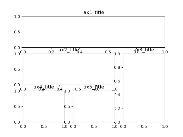
4、gridspec 1 2 3 4 5 6 7 8 9 10 11 12 13 14 15 16 17 18 19 20 21 22 23 24 import matplotlib.pyplot as pltimport matplotlib.gridspec as gridspecplt.figure() gs = gridspec.GridSpec(3 , 3 ) ax1 = plt.subplot(gs[0 , :]) ax1.set_title('ax1_title' ) ax2 = plt.subplot(gs[1 , :2 ]) ax2.set_title('ax2_title' ) ax3 = plt.subplot(gs[1 :, 2 ]) ax3.set_title('ax3_title' ) ax4 = plt.subplot(gs[2 , :1 ]) ax4.set_title('ax4_title' ) ax5 = plt.subplot(gs[2 , 1 :2 ]) ax5.set_title('ax5_title' ) plt.show()
绘图结果:
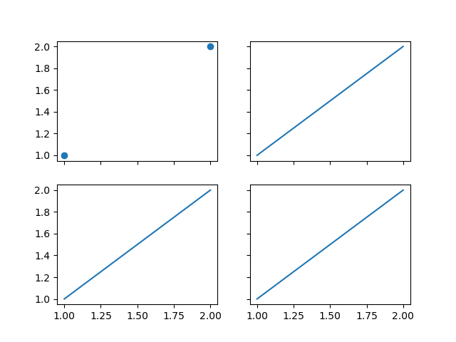
5、subplots返回参数 1 2 3 4 5 6 7 8 9 import matplotlib.pyplot as pltf, ((ax11, ax12), (ax21, ax22)) = plt.subplots(2 , 2 , sharex=True , sharey=True ) ax11.scatter([1 , 2 ], [1 , 2 ]) ax12.plot([1 , 2 ], [1 , 2 ]) ax21.plot([1 , 2 ], [1 , 2 ]) ax22.plot([1 , 2 ], [1 , 2 ]) plt.show()
绘图结果:
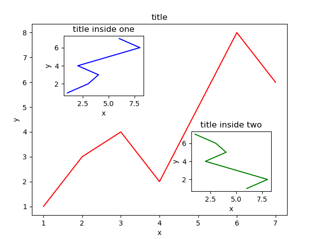
十一、图中图 1 2 3 4 5 6 7 8 9 10 11 12 13 14 15 16 17 18 19 20 21 22 23 24 25 26 27 28 import matplotlib.pyplot as pltfig = plt.figure() x = [1 , 2 , 3 , 4 , 5 , 6 , 7 ] y = [1 , 3 , 4 , 2 , 5 , 8 , 6 ] left, bottom, width, height = 0.1 , 0.1 , 0.8 , 0.8 ax1 = fig.add_axes([left, bottom, width, height]) ax1.plot(x, y, 'r' ) ax1.set_xlabel('x' ) ax1.set_ylabel('y' ) ax1.set_title('title' ) left, bottom, width, height = 0.2 , 0.6 , 0.25 , 0.25 ax1 = fig.add_axes([left, bottom, width, height]) ax1.plot(y, x, 'b' ) ax1.set_xlabel('x' ) ax1.set_ylabel('y' ) ax1.set_title('title inside one' ) plt.axes([0.6 , 0.2 , 0.25 , 0.25 ]) plt.plot(y[::-1 ], x, 'g' ) plt.xlabel('x' ) plt.ylabel('y' ) plt.title('title inside two' ) plt.show()
绘图结果:
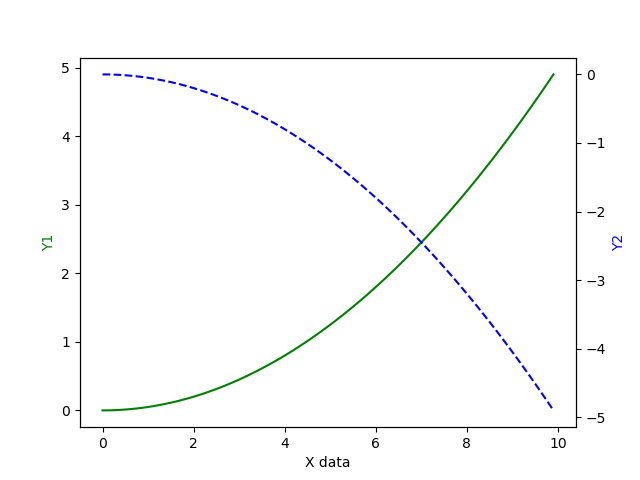
十二、主次坐标轴 1 2 3 4 5 6 7 8 9 10 11 12 13 14 15 16 17 import matplotlib.pyplot as pltimport numpy as npx = np.arange(0 , 10 , 0.1 ) y1 = 0.05 *x**2 y2 = -1 *y1 fig, ax1 = plt.subplots() ax2 = ax1.twinx() ax1.plot(x, y1, 'g-' ) ax2.plot(x, y2, 'b--' ) ax1.set_xlabel('X data' ) ax1.set_ylabel('Y1' , color='g' ) ax2.set_ylabel('Y2' , color='b' ) plt.show()
绘图结果: